
Fri Oct 27, 2017 The Sinucyli Projection
3 updates, last on Thu Jan 04, 2018
After the last update, I had exactly 199 projection images in the list of my website. Of course, these were not 199 distinct projections, since a number of projections are shown in different configurations. Nevertheless, I wanted something special for the No. 200. And I think I succeeded!
The Sinucyli projection that I added as #200 is completely new – in fact, it’s so new that it has not even been officially presented yet! Nevertheless, its creator, Daniel »daan« Strebe, kindly allowed me to show them on my website. Thank you very much, daan! : -)
The Sinucyli projection is an equal-area pseudocylindrical projection.
That’s nothing
special, there are dozens of them.
It is a blend of cylindrical equal-area and sinusoidal projection. This is also
nothing special, blending projections is a well-known procedure: the famous
Winkel Tripel, for example, is the arithmetic mean of the equirectangular
and the Aitoff projection. The Flex Projector software allows two
arbitrary projections to be mixed – including the two parent projections of
Sinucyli.
So what is so interesting about this new projection? Well, he has two special features:
- By modifying four easy-to-understand configuration parameters, the blend of the two parent projections can be customized to your own requirements. This leads to very different results (some examples follow below).
- Update! But its most important feature wasn’t known to me when I released this blogpost. The Sinucyli projection is only an example. An example for a new technique developed by Mr. Strebe, »for generating a continuum of equal-area projections between two chosen equal-area projections (…) The technique is particularly suited to maps that dynamically adapt optimally to changing scale and region of interest, such as required for online maps.« [1]
Let me emphasize: You blend two arbitrary equal-area projections, and the resulting projection is – in contrast to other methods of blending existing projections, e.g. the above-mentioned arithmetic mean – equal-area as well! A nifty feature, since equivalence is a very useful property for many purposes.
But now, let’s return to the specific example of blending cylindrical equal-area and sinusoidal projections and take a closer look at the four configuration parameters I mentioned.
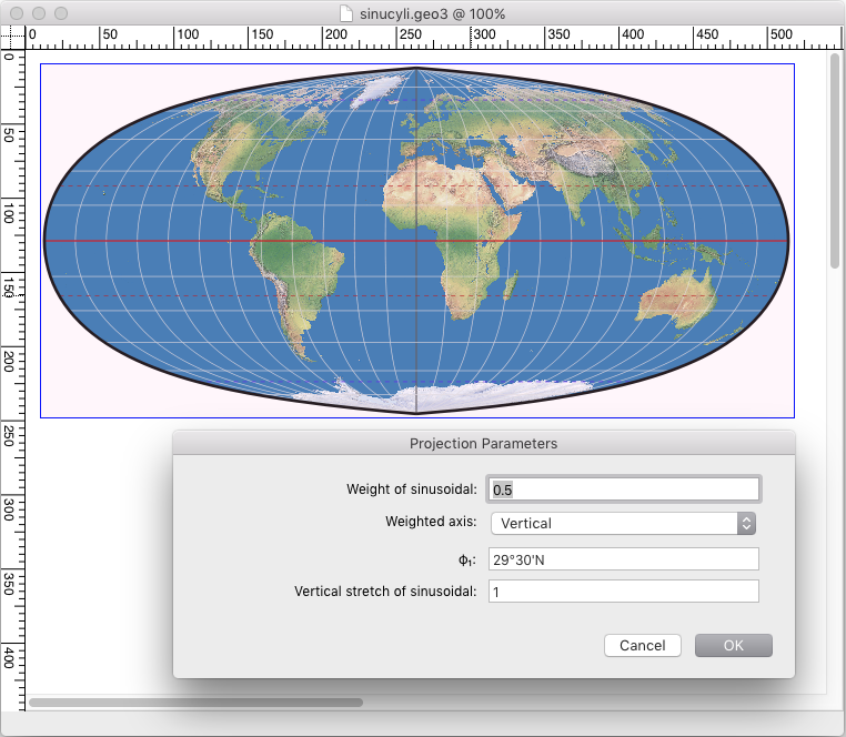
(screenshot taken from the map projection software Geocart)
Weight of sinusoidal determines the proportion of the contribution
from the sinusoidal projection. A value of 1 will result in the sinusoidal projection
as we know it – meaning there’s no blending at all.
That’s probably not what you will want to do [Update:] if you want to create a single projection;
it might be useful though for dynamic mapping and animations.
The proportion of the contribution from the cylindrical equal area projection increases towards zero.
A value of exactly 0 is not possible, but if you absolutely want to, you can
enter 0.0000001 or similar to generate a projection that is identical to the
cylindrical for all intents and purposes
again omits blending to render a pure cylindrical projection.
(Update: Entering 0 is allowed in the current beta version.)
With a value of 0.5, as shown in the screenshot,
the resultant map receives equal contribution from both source maps.
Weighted axis determines whether the above value refers to the horizontal or vertical axis of the sinusoidal projection. This doesn’t sound as easy to understand as I promised above – but basically, the vertical setting produces a projection with a pointed pole, whereas horizontal will result in a pole line.
φ1 is the standard parallel of the cylindrical projection thrown into the mix – as usual, a lower value generates will stretch the map horizontally, a higher value stretches vertically.
Vertical stretch of sinusoidal modifies the aspect ratio of the sinusoidal component. Values greater than 1 stretch vertically, values between 0 and 1 increase the width.
It may seem as if parameters #3 and #4 have more or less the same effect. In
fact, however, they are different – and I would like to show this using the
following example.
– Both maps were created with a weighting of 0.7, and with the selection horizontal
for the weighted axis.
– For the left map, a value of φ1 = 0 was selected – a value that stretches horizontally –,
which was compensated by the vertical stretch of 2.
– For the right map I did exactly the opposite:
φ1 = 80°N is stretching in north-south-direction, the vertical stretch of 0.93 counteracts this.
The two resultant maps have exactly the same height, but apart from that, they are quite different:

I think it is easy to understand what the individual values say – at least
when you have experimented with them a bit.
Now, let’s look at the three variants that I have included on the website.
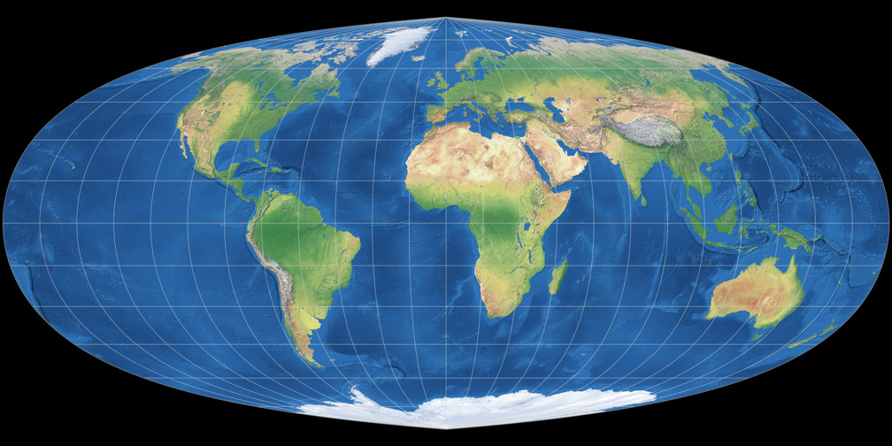

The first one is the configuration which was already shown in the screenshot
above; with the
parameters 0.5 / Vertical / 29°30´N / 1 it represents a good
starting point for your own experiments.
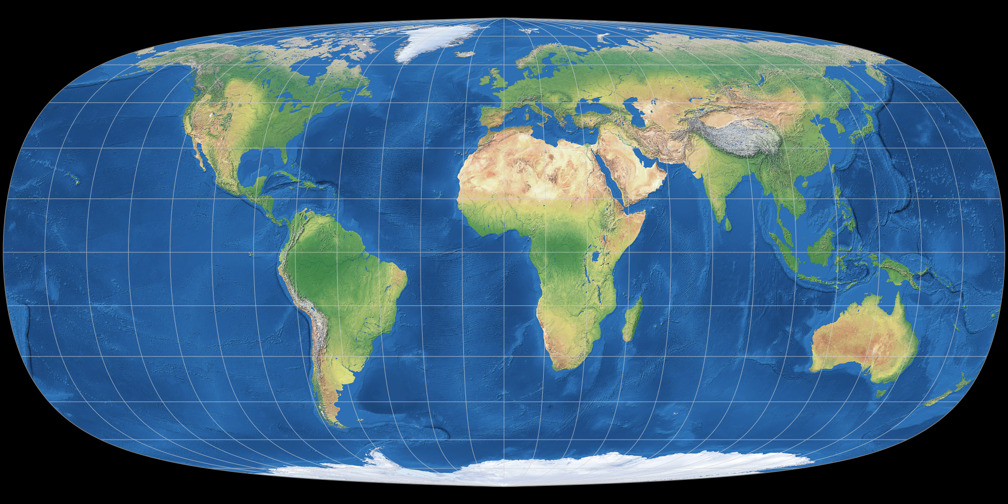
The second one (0.25 / Vertical / 29°30´N / 1.1) shows a projection approaching a
rectangular shape, but with a pointed pole.
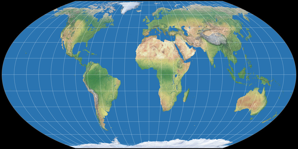
The third, on the other hand, using the values 0.8 / Horizontal / 30°N / 1,
approaches the sinusoidal, but has a short pole line.
It is not surprising that other equal-area pseudocylindricals can be approximated
using the Sinucyli projection, or that they are even identical.
For example Kavraisky V, Quartic Authalic, Eckert IV,
Thomas-MyBryde flat-pole quartic and Wagner IV each fall into one of these two categories.
And if you ask the obvious question why you should do this, instead of just referring to the original:
Well, maybe you’d like to have a projection
similar to the Eckert IV, but with a shorter pole line – or maybe you’d like the Wagner
IV with rounded corners. Such »special requests« can be fulfilled. Here is an example:

As I’ve mentioned above, a configurable projections like this is very helpful for dynamic mapping and animations.
So here is a little animation that I’ve pulled together: The parameters #3 and #4 are the same in all frames
(namely 29°30´N for the standard parallel and a vertical stretch of 1), but parameters #1 and #2 are modified:
It starts with a weighting of 1 and the weighted axis set to vertical, decreases the weighting gradually to zero,
where it switches to the horizontal axis and increases the weighting again towards 1.
Click here to view the animation!
(Sorry about some inaccuracies which e.g. make the equator blink. Next time, I’ll do better…)
Let me emphasize once again: You won’t produce surprising, unusual
results with the Sinucyli projection!
I guess this is hardly possible anyways given the thought that the
family of pseudocylindric equal-area projections probably already has more
members than any other kind.
But the ability to easily create your own
configuration is in my opinion useful enough to be seen as a valuable addition
to the world of map projections.
So, how can you use the Sinucyli projection?
Now the bad news is coming: At the moment, not at all.
It will be included in the next version of the map projection software
Geocart
– but the release date of that version hasn’t been announced yet and I guess
it’s safe to say that it’s still several months away.
As soon as daan Strebe
publishes the formula, it can of course be integrated into any other map projection applications.
I will report it here as soon as a corresponding publication is available.
Update!
Version 3.2 of Geocart has been released in Feb 2018 and offers the Sinucyli projection (among a lot of
other additional projections).
The technique has been introduced officially (see below) and thus, can be used in other map projection applications.
- ↑ Quoting from the introduction of the blending technique. The paper is available online, see daan Strebe’s note in the Geocart forum.
Comments
Due to spam posts, comments are now subject to moderation, which means they remain hidden until they are approved by a moderator.
One comment
 Except where otherwise noted, images on this site are licensed under
Tobias Jung
When setting the weighted axis to vertical, φ1 = 0 and vertical stretch = 0, the Sinucyli formula will render an instance of Foucaut’s projection with the identical value for the weighting.
Thanks for asking!