
Mon Sep 26, 2022 Two Ginzburg and Four Baranyi Projections
I’ve added six projections to my Projection Collection. Two of them are very similar to an existing projection, four are more distinct. Have a glance before I talk about them:

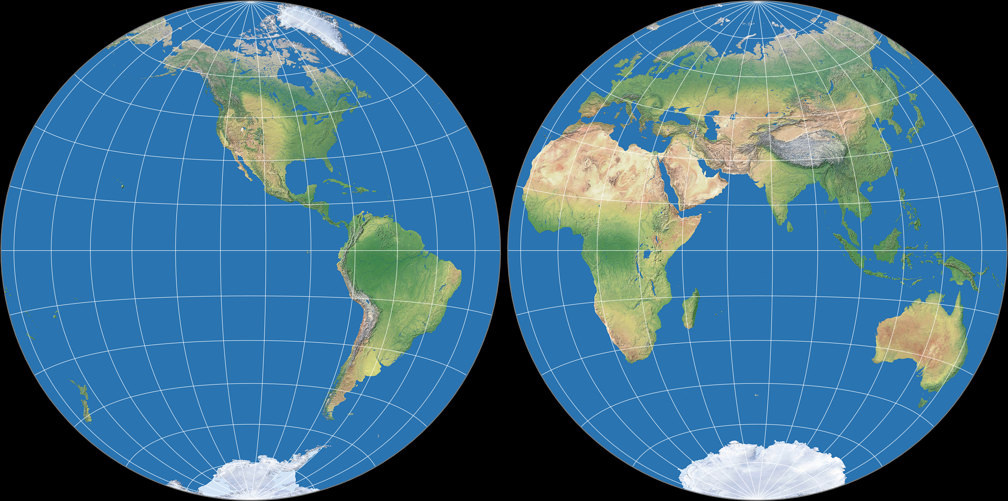


Ginzburg I & Ginzburg II
The two azimuthal Ginzburg projections are very similar, so we treat them together.

My only source about the two azimuthal Ginzburg projections is Furuti’s[1] small paragraph about them, so I can just quote him:
In 1949, Russian Georgiy A.Ginzburg proposed two azimuthal projections for hemispheres in school maps. Since Lambert’s equal-area projection compresses distances from the center of the map, causing considerable shape distortion near the borders, Ginzburg added a power term to Lambert's equations, slightly expanding the map. The result is neither conformal nor equivalent.
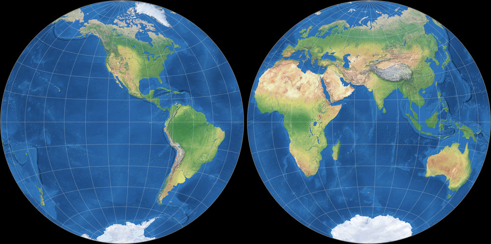
With such similarity, it makes sense to compare the projections directly with each other:
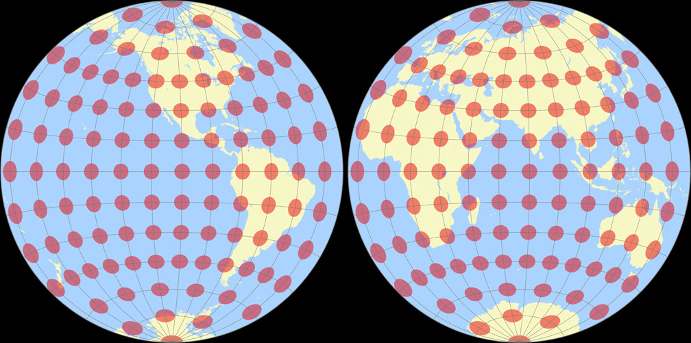
Azimuthal Equal-area vs. Ginzburg I
Azimuthal Equal-area vs. Ginzburg II
Ginzburg I vs. Ginzburg II
I’m a bit ambivalent about the results. On one hand, you could say: The deviation from equivalence is small enough not to give a false impression of the areal relationships of the countries and continents, but an improvement of the shapes at the edges of the maps is achieved. In this case, the modification would be advantageous. On the other hand, you could also say: The improvement of the shapes is so marginal that it’s not worthwhile to abandon the property of equivalence.
I tend to agree to the latter assessment, although the extra space near the edges
offered by the Ginzburg projections may come in handy if you want put to labels on your map.
Well… this is kind of an academic question anyway, since hemispheric maps are rarely
used in this day and age.
Here is the illustration of the Tissot indicatrix, and then we move on to a kind of projections you see much more often.
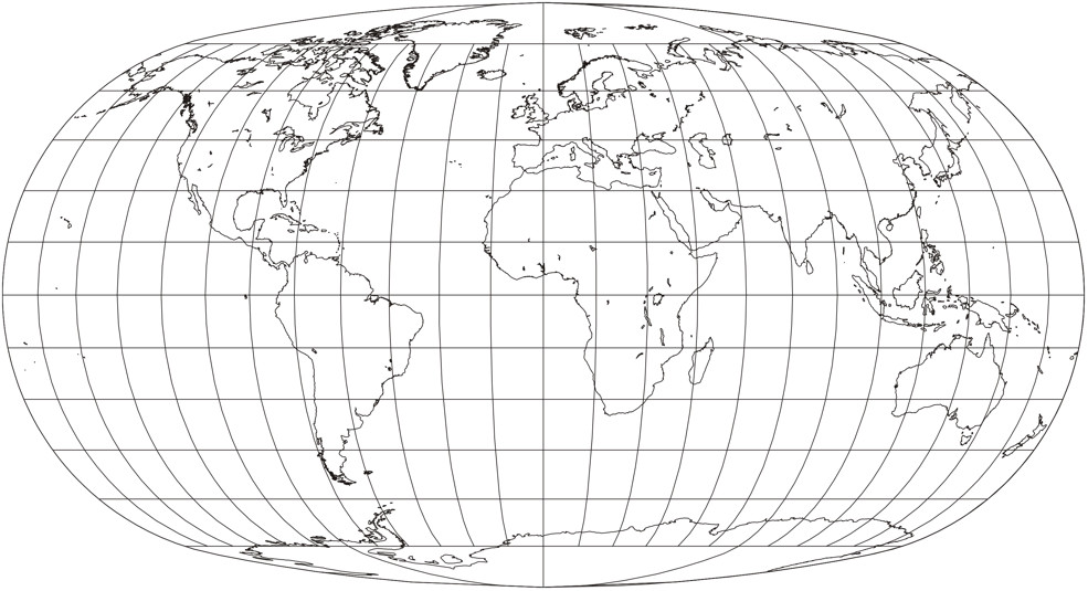
Baranyi I bis IV
In 1968, János Baranyi of Hungary presented seven projections, which were, like the poupular Robinson projection, not generated by a formula, but tabular coordinates. I’ve never read the original publication, but I think, all of them aim at a well-balanced representation of the earth (again, like Robinson). Therefore, they are neither equal-area nor conformal. I had some doubts about how to classify them, because more experienced minds than me have filed them in the pseudocylindrical group of projections[2], but only Baranyi I and II match the strict definition[3] of the term. In the end, I decided to follow the strict definition.
Regrettably, I could add only four of them to my Projection Collection because I’ve got no software
that is capable of rendering all seven. That is unfortunate because my favourite of the bunch is among
those that I cannot add. 😕
But let’s go into detail.
🌐
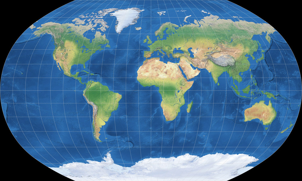
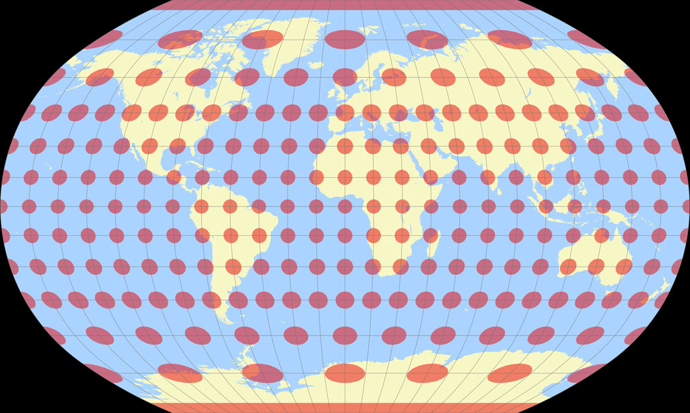
Baranyi I is a true pseudocylindrical with a pole line. Spacing of the parallels increases from the equator to the poles. It bears a certain resemblance to the Kavraiskiy VII, but in direct comparison you’ll quickly see the differences. Roughly speaking, I’d say that I’d prefer Kavraiskiy VII regarding the areal relationships and Baranyi I regarding the shapes.
🌐
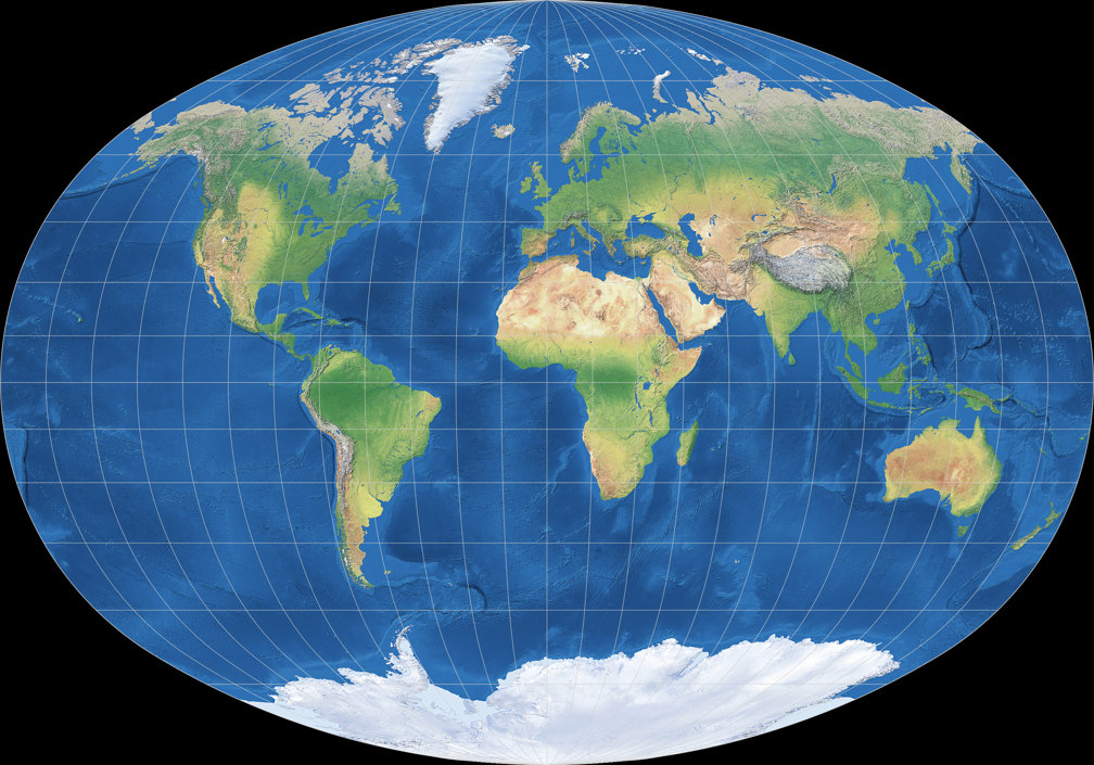
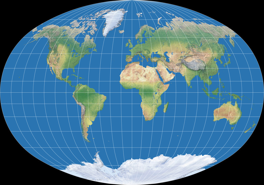
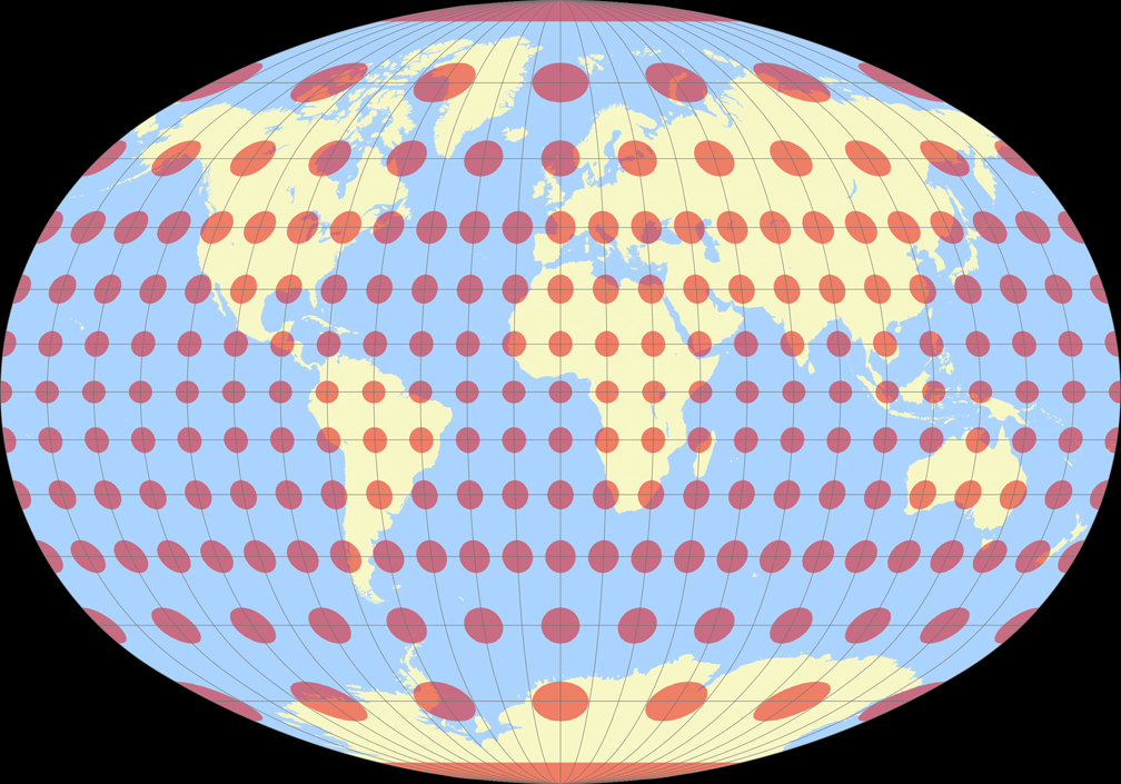
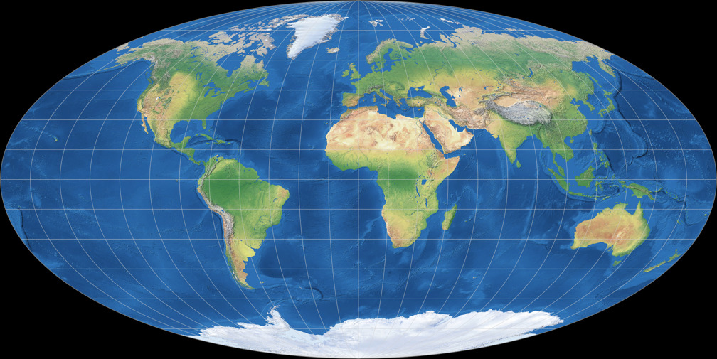
Baranyi II is a true pseudocylindrical pointed-pole projection, again the spacing of the parallels increases towards the poles. And again there is a loosely similar projection, the Fahey – compare them directly. As usual, the pointed poles lead to a much better representation of the shapes in high latitudes near the central meridian, but in turn to higher distortions near the bounding meridians. I feel that the outer shape of the projection is pleasant, but the amount of areal inflations is considerable. Therefore, I would recommend projection for decorative purposes only.
🌐
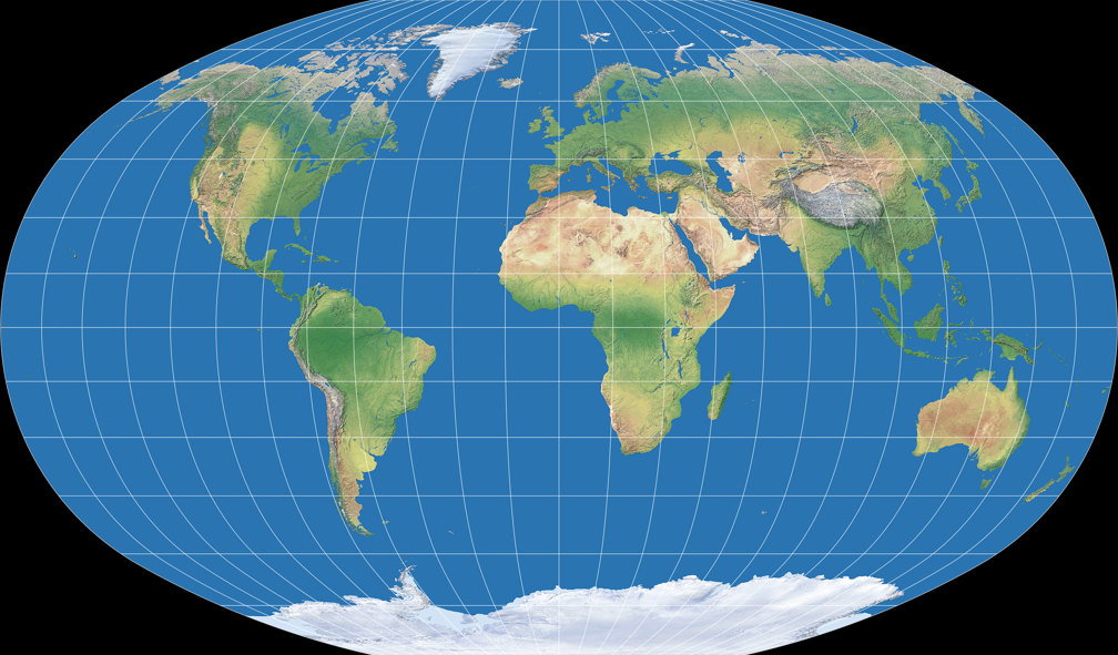
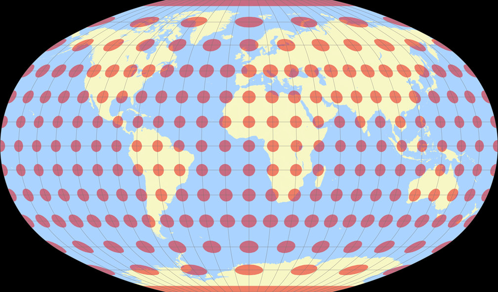
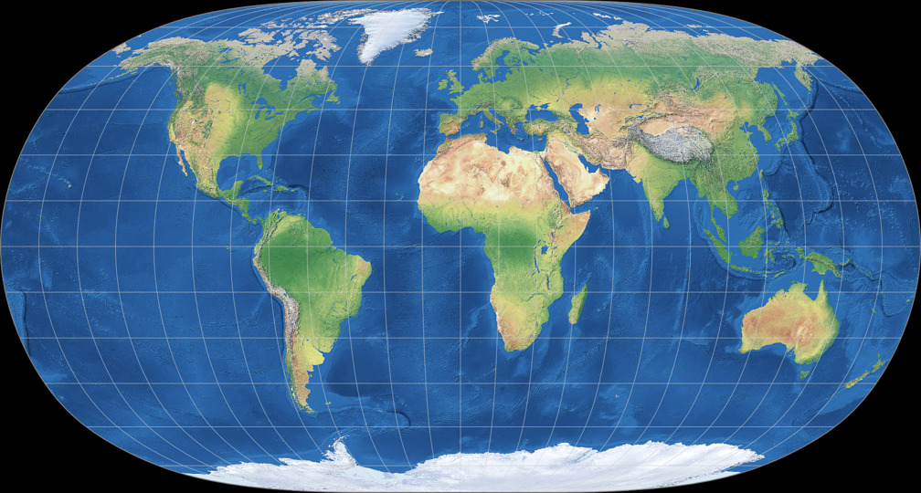
Baranyi III is – just like the ones that follow below – not a pseudocylindrical projection according to the strict definition: The distances of the meridians along a given parallel decrease from the central meridian to the boundary. The distances of the parallels to each other first increase from the equator north- and southwards and then (from approx. 50°N/S) decrease again. The inflation of the polar areas is therefore much smaller than in Baranyi I and II. A comparatively short pole line – one third of the equator’s length – ensures that they are also not stretched too much in east-west direction.
This means that in return, the angular distortions in the higher latitudes near the bounding meridians is much higher compared to Baranyi I; nonetheless, I can say that I prefer this projection over the first two, because all in all, the distribution of distortions seems more well-balanced to me.
🌐

Baranyi IV is a pointed-pole projection with an interesting combination of properties: It has clearly visible apices (unlike e.g. Natural Earth II, which might be mistaken for a pole-line projection at first glance); it avoids the “lopsidedness” of the outer longitudes in the higher latitudes (unlike e.g. Apian II); it keeps the areal inflations lower than the aforementioned Baranyi II und Fahey. That’s a rare combination.
I think it’s a very nice pointed-pole, ummm… “pseudo-pseudocylindric” projection, even if the areal inflation could still be a little lower for my taste. It’s hard for me to say whether I prefer III or IV, both have their pros and cons. In general, however, I assume that a pointed-pole projection is more likely to be accepted than one with a short pole line. Maybe that assumption is based on the fact that I have actually seen Baranyi IV in a printed atlas, where it was used for the two main world maps (the double-page physical and political maps).[4]
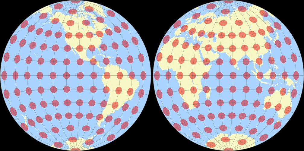
Here’s the Tissot indicatrix for Baranyi I to IV:

🌐
Regrettably, I have no software to create the images needed to add Baranyi V, VI and VII to my Projection Collection. But thanks to Anderson’s Gallery of Map Projections, I can at least show what they look like:


Baranyi V and VI (both pointed-pole projections) show a quite unusual feature: The curved meridians seem to turn into straight lines near the poles (at roughly 75°N/S). As far as I can tell from the images, the connection between the pole and ≈75° consists of two segments on projection V and a single segments on VI. I have to admit that this feature is rather displeasing to my eyes. Baranyi V has “increasing and decreasing” distances of parallels (like III & IV); on Baranyi VI the distances increase all the way up and down (as on I & II).
Baranyi VII is the only projection of the seven where the distances of the parallels
continuously decrease from the equator to the poles. Therefore, the areal inflations are smaller
than in the other six – which makes it my favourite Baranyi projection!
Although I have a hunch that if you’d measure the overall distortion values
(using e.g. the Airy-Kavraiskiy criterion), it’ll turn out that Baranyi IV
comes up with a better result than VII.
But fortunately, I don’t have to care about that. 😉
’nuff said.
References / Footnotes
- ↑ Cited from Carlos Furuti’s website from the Internet Archive.
- ↑ All Baranyi projections are cited as pseudocylindricals in the libproj4 manual by Gerald I. Evenden, the Map Projection Gallery by Paul B. Anderson, G.Projector’s List of Map Projections, and in their mention in the description of the Robinson projection in the Geocart manual. In Flattening the Earth, John P. Snyder introduces them as “non-equal-area pseudocylindrical-like projections” (p. 216) to then list them in the pseudocylindrical section of the table on p. 281.
- ↑ The strict definition of the term “pseudocylindrical” is for example given in Wikipedia (… meridians are equally spaced along a given parallel) or daan Strebe’s Map Projection Essentials, see section “Mathematical projection”: (…) being those projections with meridians curving toward the poles and straight, scale-invariant parallels (the scale of any given parallel is constant along its entire length).
- ↑ Diercke Drei Universalatlas, Westermann Schulbuchverlag GmbH, 1. Auflage 2001.
Comments
Due to spam posts, comments are now subject to moderation, which means they remain hidden until they are approved by a moderator.
2 comments
Alexandre Canana
Robert Schmunk
Unfortunately, there are multiple versions of the PDF out there and at the moment I do not know where to obtain the 2008 version that I have. I think I downloaded it from Evenden's website, which is of course now long gone. There is a 2005 version at http://libproj4.maptools.org
FWIW I implemented Baranyi I, II and III this this past spring using Zelenka's method. But Zelenka's Baranyi IV differs from that of Evenden (which I coded up 4 years ago) and of Györffy and Márton. The latter two versions of Baranyi IV are not identical but are very, very close.
Robert Schmunk
Tobias Jung
Kind regards,
Tobias
Robert Schmunk
Robert Schmunk
The Baranyi V, though, has somewhat more clipping at the poles, so looks trickier.
Robert Schmunk
Tobias Jung
Robert Schmunk
Was comparing the different formulations for the Baranyi IV again, and it looks like almost entirely something to do with the approximation for longitudex, with the maximum difference occurring at +/- 90 degrees from the center meridian. Visual comparison show almost no or none difference in placement of the parallels. As my current code is based on two sources that use almost exactly the same formulation, I'm sticking with it for now.
 Except where otherwise noted, images on this site are licensed under
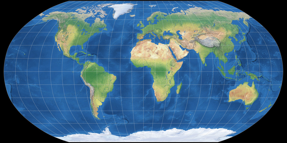
Alexandre Canana