
Fri Jan 15, 2021 More Umbeziffern for d3-geo-projections
In June 2018 I introduced the customizable Wagner VII in an implementation
for d3-geo-projections. Now, I’m going to up the ante
and add customizable variants of Wagner I/II and a few projections with equally spaced parallels (along the
central meridian), including two different approaches for Wagner III.
I couldn’t have done it without lots of help by Peter Denner. Thanks a lot, Peter! 🙏
However, there are a few differences to the implementation of the Wagner VII.
This blogpost is mainly about the Whys – Why are the differences? Why are there (seemingly) redundant
parameters?
If you’re less interested in these question, but more in the Hows – How can I customize the projections? –,
then only read the following Outline and then head over to
Customizable Wagner Projections using d3-geo – Seven Of Nine.
Note that I’m proposing new functions for d3-geo-projections here! They are not part of the current distribution, they are not fully tested, there might be bugs and they still might be changed!
Outline
For better understanding, we take a look back:
The existing implementation of the customizable Wagner VII/VIII allows to modify four parameters: The length of the pole line,
the curvature of parallels, the amount of areal inflation and the aspect ratio of the axes (equator towards central meridian).
The source code can, for example, look like this:
d3.geoWagner()
.poleline(65)
.parallels(84)
.inflation(25)
.ratio(200)
poleline() accepts values from 0 (pole line length equals equals length) to 90 (pointed pole);
parallels() values from 0 (parallels are straight lines) to 180 (strong curvature);
inflation() from 0 (no inflation, i.e. equal-area) to 99.999;
and ratio() sets the aspect ratio of the axes, namely the percentual length of the equator relative to the central meridian.
Basically each number greater than 0 and lower than 1000 is allowed, but the range of sensible values is of course much smaller.
Let us now turn to the new, proposed functions. As you will see, there are similarities and differences.
🌐
Example of the proposed customizable Wagner I/II:
d3.geoWagner2()
.poleline(0.5)
.inflation(20)
.ratio(200)
For inflation() and ratio(): See above.
poleline() however is noted as a value between 0 (pointed pole) and 1 (pole line length = equator length).
The reasons will be given below.
🌐
The proposed customizable Wagner III:
d3.geoWagner3()
.poleline(0.5)
.ratio(200)
.phi0(40)
The parameters poleline() and ratio() work as on the Wagner I/II –
on top of that, you can set standard parallels using phi0(), which also effects
the aspect ratio. Again, this will be explained below.
🌐
And last but not least, the customizable Wagner ESP which renders projections with equally spaced
parallels:
d3.geoWagnerEquallySpacedParallels()
.parentProjection(9)
.poleline(70)
.parallels(50)
.ratio(200)
.xfactor(100)
All Wagner projections are derived from a parent projections. While the parent is fixed on the other variants mentioned here,
you can select it on the Wagner ESP from a fistful of options – that’s what the parameter .parentProjection() is for.
.poleline().parallels().ratio() – these are set according to the Wagner VII/VIII mentioned above.
And then we have .xfactor() which, like .ratio() changes the aspect ratio of the map.
The reason, as you will guess, is explained below.
🌐
Aaaand there’s also the Apian II. No parameters, just plain and simple
d3.geoApian2().
🌐
So much for the outline. If this is enough information for you – as I’ve said above,
you can now
see and try examples.
For closer information, read on.
Umbeziffern – What was that again?
I’ve talked about Umbeziffern several times, most recently… well, again, in June 2018.
Let’s recap: Take a part of the graticule of some parent projection, which is defined by a limiting parallel and a
limiting meridian; project the whole Earth to this part, bring it to the scale of the original projection and
stretch it horizontally. The limiting parallel affects the new projection’s length of the pole line and
the limiting meridian affects its curvature of parallels.
Wagner also added a way to determine the areal inflation of the new projection.
For example, in the
Wagner-Böhm I
the limiting parallel is set to 65° N/S, the limiting meridian to 84° E/W,
the areal inflation to 25% (at 60° N/S, a reference parallel that is hardcoded in the script) and the
axial ratio to 200% (= the equator is twice as long as the central meridian).
This projection is noted in the d3 scripts like this:
d3.geoWagner().poleline(65).parallels(84).inflation(25).ratio(200)

Lambert’s azimuthal equal-area projection with emphasized limiting parallels/meridians (left) and the resulting Wagner-Böhm I
For Wagner VII/VIII, the parent was the azimuthal equal-area projection in the equatorial aspect. But all nine projections that named after Wagner were obtained by the use of Umbeziffern using different parent projections … and sometimes, a slightly different approach.
We’ll go into detail now.
The customizable Wagner I/II
Just like Wagner VII and VIII, Wagner I and II are generated from the same formula, the only difference is the amount of areal inflation which is set to zero on the Wagner I, rendering an equal-area map. On the original projection No. II, Wagner decided to set an areal inflation of 20% (at 60° N/S as mentioned above). The notation of my implementation looks like this:
d3.geoWagner2().poleline(0.5).inflation(20).ratio(200)
The parameter .parallels() is missing here:
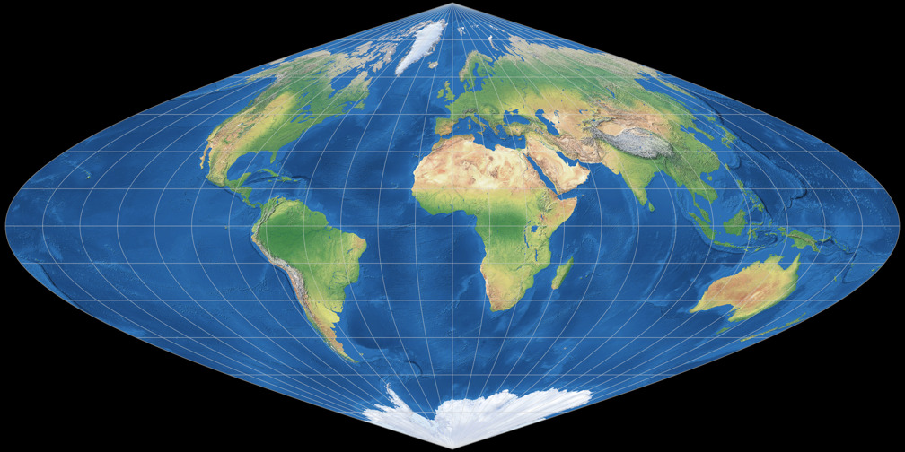
Wagner I and II are derived from
the sinusoidal projection
– a pseudocylindrical projection with its typical straight parallels.
This property is maintained, thus there’s no parameter to set the curvature of parallels.
But what about .poleline(0.5)? Certainly the limiting latitude isn’t at 0.5° N/S? No, of course not.
For the projections that are nowadays known as Wagner I to VI, Herr Wagner chose a different approach:
He determined the length of the pole line relative to the equator’s length, beginning the development of the final formula
with the variable c = 0.5 which renders a pole line that is half as long as the equator. Note that this indeed
is just a different way to express the desired length – Wagner did not forget to mention that a value of 0.5 corresponds
to a limiting parallel at 66,42°. But in the formulae that convert the input parameters to the final projection formula, he
used the aforementioned value of 0.5 for c.[1]
So if I know that c corresponds to a certain limiting latitude, why don’t I use that to keep the
notation consistent?
The thing is, I’m bad at math.
I can transcribe a formula, e.g. from C syntax to JavaScript, which I did for the final formula – for the
Wagner I/II, my template was Evenden’s C implementation of the Wagner I.[2] For the conversion of the input parameters to the values that are passed to the final formula, I transcribed
the steps that are given by Wagner himself.
What I can’t do is rewriting a formula. I lack the knowledge in math to say: “Oh, let’s replace
that c variable with a proper ψ1 for the limiting parallel…”
So I simply had to keep the relative size of the pole line. I have to admit that this bugs me a bit.
On the other hand, when both equator and pole line are straight lines, maybe it’s even more intuitive
to use the aspect ratio of those two lines instead of the more abstract limiting parallel.
So now you might ask: “Then why don’t you at least use a percentual value like you do on the aspect ratio of the equator towards
the central meridian”? – Good question, let’s go through this:
Corresponding to .ratio(), you could write .poleline(200) to indicate that the equator is
twice as long as the the pole line. But what about a pointed pole? In this case the
pole line length equals zero, and 200% or 1,000% or 78,435% of 0 still is 0. It doesn’t work out.
What about the other way round, writing .poleline(50) to indicate that the pole line is half as long
as the equator? This of course is the same thing as using 0.5 so it works out, and at least we now
have a percentual value again instead of a multiplier. Yes – but on the Wagner VII/VIII, .poleline(80)
generates a very short pole line, while on the Wagner I/II it would generate a very long pole line. If you increase that
value, the pole line approaches a pointed pole on VII/VIII but it would approach the equator’s length on the I/II.
I found this to be too confusing.
With a .poleline() value that’s between 0 and 1 on the Wagner I/II, you can at least see at the
first glance that something differs from the notation of the Wagner VII/VIII.
Granted, it is a bit of a nuisance that the notation differs.
But on balance, I think this is the best solution.
(Maybe renaming this parameter is a good idea, but I couldn’t come up with anything less confusing. I’m open
to suggestions.)
If you want to see the possible result of the customizable Wagner I/II head over to
the interactive demo.
The customizable Wagner III
The parent projection of the Wagner III is the
Apian II,
a pseudocylindrical projection with equally spaced parallels. So again, we can omit the parameter
.parallels() because there is no curvature – but this time, there’s no .inflation()
parameter as well: Changing the areal inflation would result in a projection that doesn’t have
equally spaced parallels anymore.
So far, we’re down to the parameters .poleline().ratio() – the former being noted as
value between 0 and 1, like on the Wagner I/II.
In order not to make it too easy 😉 we’ll add a new, confusing parameter: .phi0().
phi0 is, in the d3 scripts, the usual way to write φ0,
and that’s the standard parallel. The standard parallel is the one that is deemed to be at the right scale.
In effect, changing phi0 changes the map’s aspect ratio…
Huh? What? But that’s what the .ratio() parameter is for, isn’t it?
Well, yeah. Kind of. Let me eloborate:
Wagner described both methods. He used the variable p = 0.5 to determine the
aspect ratio of the axes, developed the final formula and in the end, added the option
to set a standard parallel. I always understood this as an alternative: When you want to change the aspect ratio
of the map, either modify the p or leave it at 0.5 and set the
standard parallel. And recently, I was a baffled when I stumbled across a paper which modified both parameters…
The paper in question is of course the one by Nedjeljko Frančula[3] which I mentioned recently. Let me repeat that Frančula optimized distortion values of various projections (among them, the Wagner III). He used both ways of setting the aspect ratio which makes sense in this regard.
Well, try the interactive demo!
There, you can see that
d3.geoWagner3().poleline(0.5).ratio(147).phi0(0)
and
d3.geoWagner3().poleline(0.5).ratio(200).phi0(40)
are identical (but note the different scale in the “Customize Map” section). Or call
d3.geoWagner3().poleline(0.69).ratio(195).phi0(44)
to see one of Frančula’s optimized variants.
The customizable Wagner ESP – Umbeziffern with Equally Spaced Parallels
About three years ago, I presented the WVG-9, which was a quick&dirty hack of a customizable Wagner IX.
I always wanted to clean it up, but never actually did it. Until Peter Denner recently pointed out that it had
a bug. I tried to fix it but I kept failing. So Peter jumped in and not only fixed the bug, but also showed me
that the function could easily be used to apply the Umbeziffern to other projections with equally spaced parallels
that already are part of the d3-geo-projections distribution.
While this is based on my original code for the WVG-9, most of the work was done by Peter.
First off, we have a new parameter to set the parent projection:
.parentProjection()
Unfortunately, we have to pass a numerical value here – I’d prefer to set the name of
the parent projection, but that’s not possible.[4] So here’s the current list
of parent projections, the existing Wagner projections that are derived from them,
and the numbers you have to provide to use them. As you can see, it also
includes the Wagner III that we’ve covered above. I’ll come back to this later.
| Parent Projection | Variant of | Call with |
|---|---|---|
| Sinusoidal | Wagner III | .parentProjection(3) |
| Apian II | Wagner VI | .parentProjection(6) |
| Azimuth. Equidist. | Wagner IX | .parentProjection(9) |
| van der Grinten IV | — | .parentProjection(10) |
| American Polyconic | — | .parentProjection(11) |
| Nicolosi “telophasic” | — | .parentProjection(12) |
| Rectangular Polyconic | — | .parentProjection(13) |
For the Wagner projections I just translated the roman into arabic numerals, and
for the others I just continued counting at 10…
I’m really not fond of this approach, but I didn’t know how to do it in a better way.
.poleline() and .parallels() use, like on the Wagner VII shown in the beginning,
the limiting parallels and meridians of the parent projection. .ratio() works like on all examples
shown here. But again, I’m adding a new parameter which seems to bei redundant at first:
.xfactor() – what’s that?
.xfactor() (which I named that way because I could not think of anything else) compresses or stretches
the width of the map. The noted value is the percentual width of the width that is determined by .ratio().
The reason to introduce that parameter is very much like we’ve had before: It’s the way Wagner did it. And for a good
reason, from the perspective of the time: He developed the formula using the variable p = 2
(corresponds to our .ratio(200)), arrived at the final formula and then said that you can improve
the distribution of distortions by multiplying all the x-values with the factor a < 1 and
showed an example with a = 0,88 which results in a projection that is close to Winkel Tripel Bartholomew.[5]
This made sense because at that time, they of course had no computers.[6] So if you have a table with the cartesian coordinates – and Wagner provided one in his textbook –, you just had to multiply all the x-values with the factor you preferred, and you’re done. That’s a lot less work than to calculate the table again with a different value of p.
But today, we’ve got computers, and since
.poleline(70).parallels(50).ratio(200).xfactor(88) renders the same map as
.poleline(70).parallels(50).ratio(176).xfactor(100) (again, apart from the nominal scale)
I already had decided to drop the .xfactor() and let the width be determined by .ratio() only.
But – as you might guess already – Frančula again used both parameters and since I wanted to reproduce
his variants including their calculated distortion values as accurately as possible, I had to keep them both.
Again, I’m inviting you to visit the
visit the interactive example:
You’ll see that when you change .ratio(), the map will be stretched horizontally and at the same time,
compressed vertically (or vice versa) – it’s an area preserving modification (an affine transformation), the
amount of areal inflation doesn’t change. On changing .xfactor() however, the map gets stretched or compressed
horizontally only, which results in a change of the nominal areal inflations.
Note that it is not required to actually use both values – it’s possible to omit one of them which then will
drop back to the default values.
Besides the interactive demo you can also use the WVG-9 which has been renamed to WVG-ESP. In the interactive example you can drag a few sliders and the projection will be updated on-the-fly, while the WVG-ESP reloads the page each time you try different parameters. On the other hand, the WVG-ESP allows up to three decimals on each value, while the interactive example is restricted to half integers. Moreover, the WVG-ESP offers a few more options.
… and in passing: The Apian II
As I’ve said above, the Wagner ESP uses formulae of parent projections that already are included
in d3-geo-projection. For the Wagner VI, the parent projection is Apian II which wasn’t available
– so Peter wrote it.
The Apian II itself has no parameters, so you just call it with d3.geoApian2().
Summary
I’ve proposed three additional variants for customizable projections (on top of the one that already existed)
based on Wagner’s transformation method of Umbeziffern in an implementation for d3-geo-projections.
Some of them have different parameters than others, but that’s the nature of the beast.
It’s more annoying that the notation of parameters differs in some examples
although they actually they actually do the same.
This probably could be fixed by someone with more knowledge of the mathematics.
Some parameters are redundant, they could be dropped unless you go for minimal distortions according to a given metric.
On the other hand, both the deviating notations and the redundancies can be helpful if you want to
render an existing projection exactly as it was specified by its author.
In my opinion, the customizable Wagner I/II is not very interesting, because sinusoidal meridians do not seem to be favoured by a lot of people, and there already are a hell of a lot of pseudocylindrical projections… At best, the option to freely set the amount of areal inflations might be of some interest.
The customizable Wagner III can be helpful if you want a projection with equally spaced parallels that follows the mathematical description as given by Frančula. But it is kind of obsolete because its (differently described) included in the Wagner ESP.
The Wagner ESP however is very interesting, mainly thanks to Peter Denner who showed me how to apply the transformation to other parent projections. I really love that bit!
The only thing better would be to able to apply the transformation of the Wagner VII/VIII to other parent projections since it has the option to set the areal inflation… which theoretically is possible but not to me.
For examples of projections rendered with the proposed functions, incl. the interactive exampes,
and the source code for integration in d3-geo-projections, see
Customizable Wagner Projections using d3-geo – Seven Of Nine.
Supplement
I had this blogpost almost finished, when Peter Denner again sent me something:
A function to render the Canters’ optimization of Wagner IX.
I’ve added it to the source code
because it might be interesting to some people (as myself) but probably it’s not necessary to add it
to the official d3-geo-projection plug-in: Canters’ projection can of course be rendered with the Wager ESP
if you know the correct values. Canters chose a somewhat different mathematical approach
so I always failed to find them, so I
presented approximations only in the WVG-9.
Peter’s function now enabled me to find the values. 😁
They are:
d3.geoWagnerEquallySpacedParallels()
.parentProjection(9)
.poleline(67.131)
.parallels(86.562)
.ratio(206.7978)
.xfactor(80.7486)
I’m using up to four decimals here to render it as close as possible.
Note that the
interactive example showing Canters’ optimization
still is an approximation because that example is restricted to half integers.
The WVG-ESP however uses the decimals
shown above. I do think that this is close enough to call it the real thing, not an “approximation”.
Footnotes
- ↑ Wagner, Karlheinz: Kartographische Netzentwürfe. Leipzig 1949/Mannheim 1962, p. 180 – 181
- ↑ Gerald I. Evenden, libproj4, cartographic projection library.
- ↑ Nedjeljko Frančula: Die vorteilhaftesten Abbildungen in der Atlaskartographie. Bonn 1971. Available at researchgate.net (German)
-
↑
The d3 script include a function calles
mutate()which can be used to change certain parameters of a projection. Since it usually modifies standard parallels etc. it only accepts numerical values. It’s possible that there’s a different way to do this. But I don’t know how… - ↑ Wagner 1949/1962: p. 214 – 217
- ↑ They had no computers: Of course I’m talking about the electronic gadget here. I know that back in the old days, the term computer referred to a human whose job was … to compute.
 Except where otherwise noted, images on this site are licensed under
Comments
Due to spam posts, comments are now subject to moderation, which means they remain hidden until they are approved by a moderator.
More info
Be the first one to write a comment!