Mon Jan 24, 2022 A Fistful of Asymmetric Projections
In December, I introduced two asymmetric projections, Weia Reinboud’s Cupola projection and my own Asymmetric Wagner VII.b. The latter was a composition of the northern and the southern hemispheres rendered with different configuration parameters, which then were put together at the equator. I ran into three certain problems:
- In the first version I came up with, there were discontinuities in the distribution of distortions along the equator.
- I was (for me) a somewhat time consuming task to find configurations for the two hemispheres that will fit together seamlessly.
- And in the end, it turned out that the asymmetrical variant may not have had any advantage at all compared to a corresponding symmetrical variant.
But a while ago, it occurred to me that there is a family of map projections
that are customizable and enable me to create asymmetric projections
that will always fit together perfectly at the equator, without
any discontinuities or any hassle to find the right parameters.
So problem #1 and #2 were solved, and regarding #3 – we’ll see.
Please note that the Cupola projection has a very specific goal and was mathematically developed to reach it. The projections I’ll show today are far less specific: Like the asymmetric Wagner VII.b, they are just trying to reach a distribution of distortions that is advantageous to the continental areas of both hemispheres (except Antarctica).
Asymmetric variants of the 1992 Strebe projections
About three and a half years ago, I wrote a blogpost regarding
Strebe’s equal-area projections of 1992 – please read it for
detailed information about the projections. For now, just let me quickly summarize:
They are transformations of six existing projections
(Sinusoidal, Mollweide, Hammer, Kavraiskiy V, Snyders’s minimum-error pointed-pole and flat-pole),
that can be configured by a parameter which controls the curvature of the (pseudo) pole-line
called μ – the ancient Greek letter Mu [mŷː] –
in Geocart or Bonne φ1 in Strebe’s paper of 2018.[1]
The μ is a latitudinal value, the allowed range differs on the various projections,
e.g. on the Strebe-Mollweide it has to be between 43°N and 29°S; each value will render a different result.
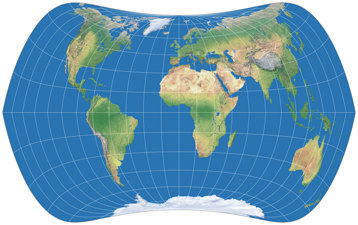
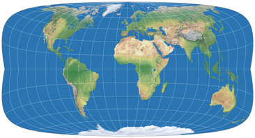
Let’s look at the said projection, two times with a μ of 24°,
but with 24° North in the first and 24° South (as shown in the frontispiece of my
2022 map projection calendar)
in the second image:
Both show kinks in the meridians at the equator which is typical for this family of projections.
Apart from that, they are quite different – but there is a thing that was quite
interesting to me:
If you render both variants at the same nominal scale, they fit together perfectly at
the equator! And this holds true for all of Strebe’s 1992 projections.
The tedious search for the right values, which enable me to construct a
continuous map, is thus completely eliminated.
All I have to do is:
– render the northern hemisphere with a northern value of μ;
– render the southern hemisphere with the same southern value;
– but the two hemispheres together.
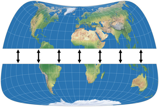
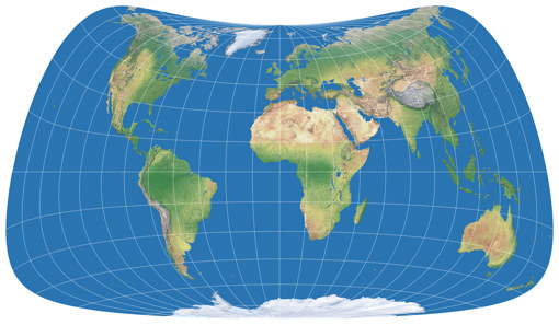
… and voilà, here’s the first projection of the series, Strebe-Mollweide Asymmetric 24:
The first positive effect: The kinks at the equator are gone, the graticule lines now merge continuously from one hemisphere to the other. So, what about the above mentioned problem no. 3 that I had with the asymmetric Wagner VII.b? See for yourself, here’s the symmetric Strebe-Mollweide with μ = 24°N and once more with μ = 24°S – and in between, the asymmetric variant that was composed of them. While again there are some parts of the northern hemispheres that are better off on the “southern variant”, summa summarum I think you really can say that this time, both hemispheres are served well:
🌐
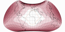
After I had found this out, I of course tried out whether an advantageous north-south combination could also be found for other projections of the series. I did not succeed in this for Strebe-Hammer and Strebe-Sinusoidal (which doesn’t mean that it doesn’t exist but merely that I didn’t find a configuration that I liked). But the Strebe-Kavraiskiy V with μ = 20° N/S is not too bad:
Alright, everything above roughly 75°N looks a bit like it’s being sucked into a hoover which
is located at the north pole…
However, with its modest amount of asymmetry, the almost straight pseudo pole line
(“pseudo” because there is no pole line here, but a pointed pole) and an outer shape
which moves towards a rectangular shape, it might be a fitting example
in case you don’t want to go too far out on a limb.
Comparing the three variant again, I think the situation is much like on
the Strebe-Mollweide above:
🌐
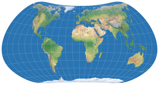
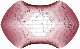
The next one is the only one among the projections shown today that has an actual pole line. It’s the Strebe-Snyder Flat-Pole, again with μ = 20° N/S. Since it looked too wide to me, I added an area-preserving vertical stretch[2] by 1.05:
Honestly, I’m not that fond of this variant – it shows the typical problem of an equivalent projection with a long pole-line: It makes the polar area look quite “squished”. I thought about dismissing this one, but I wanted to keep a pole line projection within the mix. But more importantly: New Zealand’s position in the “corner” of the map (in equatorial aspect, centered to or near the Greenwich meridian) has the effect that in the other projections of this series, the amount of angular distortions varies significantly across the country. For example, on the Strebe-Mollweide and Strebe-Kavraiskiy variants shown above, the max. angular distortion at the northernmost tip is at roughly 20° but at the southernmost tip, it’s at ≈45°. But on this Strebe-Snyder Flat-Pole configuration, the range is 22° to 29° – which still is considerable for a rather small area, but an improvement nonetheless.
It’s also noteworthy that among the whole bunch, this is the projection that has the largest area of land which remains under an angular deformation of 20°. Which is a good reason to keep it, despite my aesthetic reservations.
🌐
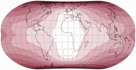
Finally compositions of the Strebe-Snyder Pointed-Pole.
The first one is combining the hemispheres with μ = 20° North/South.
Despite having a pointed pole, it’s not that far away from Wagner VII,
the probably best-know lenticular equal-area projection with a pole line
(only in the sense of the “general look & feel”, of course there are obvious differences):
Strebe-Snyder Pointed-Pole Asymmetric 20 vs. Wagner VII
The ratio of the main axes is almost exactly 2:1, which also holds true for the Strebe-Kavraiskiy above. The latter has the better southern hemisphere and on the northern hemisphere, large parts of the continents are also treated better. However I have to say that I find the Strebe-Snyder PP 20 more pleasing to the eye.
🌐
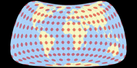
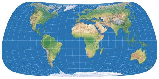
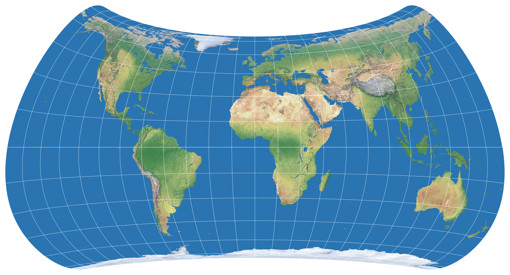
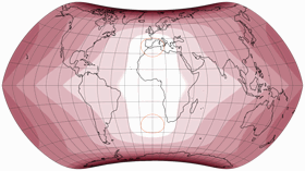
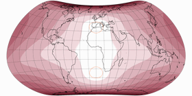
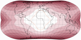
And then, I tried the Strebe-Snyder Pointed-Pole again with a more pronounced asymmetry, namely μ = 26° N/S. Again, I slightly adjusted the aspect ratio again, but this time I stretched it horizontally by 1.05 (again, using an area-preserving stretch).
The strong curvature of the northern pole line may not be to everyone’s liking,
but I do think that it improves the distribution of distortions for (most of) the landmasses
on both hemispheres.
This is my personal favorite among the projections presented here.
No Discontinuities
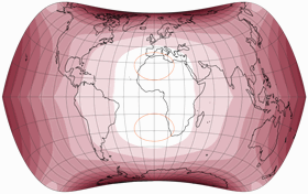
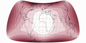
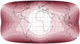
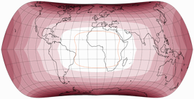
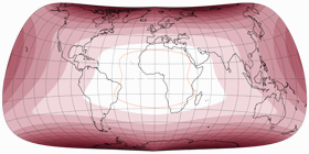
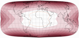
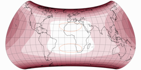
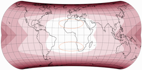
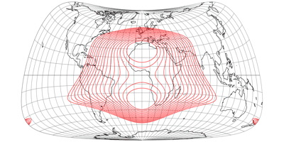
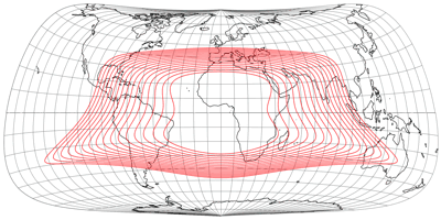
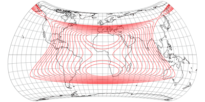
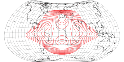
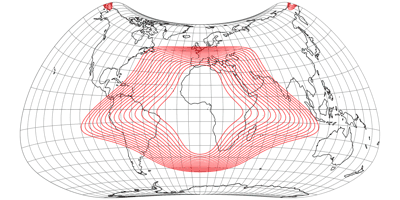
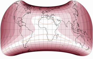
It was actually already clear from the distortion graphs shown above, but in order to show that the compositions do not show any interruptions in the distribution of the distortions at the equator, here are the plots with isolines of the angular deformations from 5 to 20°:
Résumé
Strebe’s 1992 series of equal-area projections provide an easy way to experiment with asymmetry, without any hassle or the need for any calculations. The results presented here certainly aren’t spectacular, but in my opinion, quite employable. Regrettably, I think none of my configurations has such favorable distribution of distortions as the Strebe Asymmetric 2011. But basically, that was to be expected…
References
-
↑
Strebe, Daniel (2018):
A bevy of area-preserving transforms for map projection designers.
available at researchgate.net - ↑ An area-preserving stretch means that you multiply the height with a specific value, and the width with the reciprocal of it (or vice versa); e.g. if the height is multiplied with 1.05, the width gets multiplied with 1/1.05 = 0.95238095.
Comments
Due to spam posts, comments are now subject to moderation, which means they remain hidden until they are approved by a moderator.
One comment



 Except where otherwise noted, images on this site are licensed under
Tobias Jung
Alexandre Canana
Alexandre Canana