
Fri June 16, 2023 Adams, Baranyi, Winkel-Snyder
After five months, there are finally new entries in my projection collection. And fittingly, there are five of them. 🙂
Another conformal projection by Adams

Three years ago, I presented Adams World in a Hexagon in my projection calendar, using an uncommon projection center. A few weeks ago, I received a message asking me to add it to my Projection Collection, preferably in the polar aspect proposed by Adams.
Ummm?
Haven’t I already done that?
No, I haven’t. I will do so here and now.
Thank you, Henry, for bringing this to my attention! 🙏
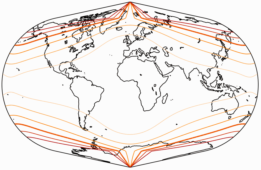
Here’s the visualization of the areal inflations, normalized to the value at the central point.
The lines represent an enlargement by the factor
1.2; 1.5; 2.0; 2.5; 3.0; 3.5; 4.0; 4.5; and 5.0:

Three hitherto missing projections by Baranyi
Last year, I added four projections by János Baranyi to my Collection and noted that there were three more, of which I unfortunately cannot generate images. there are three more, but I couldn’t generate images showing Well, guess what – now I can! Here are Baranyi V, VI and VII:


You can read all I’ve got to say about them in the blogpost I’ve linked to above (aah, what the heck, here’s the link again), so there’s no need to get chatty here; and I can get straight to the important point:
I can present visualizations of distortions for all seven Baranyi projections! And I can tell you, that was some piece of work, because… *cough* Alright, probably it was a lot of work indeed, but not for me. Once more, Peter Denner provided them for me. Perhaps I should mention it in future blog posts when I don’t owe Peter any thanks for once? 😉
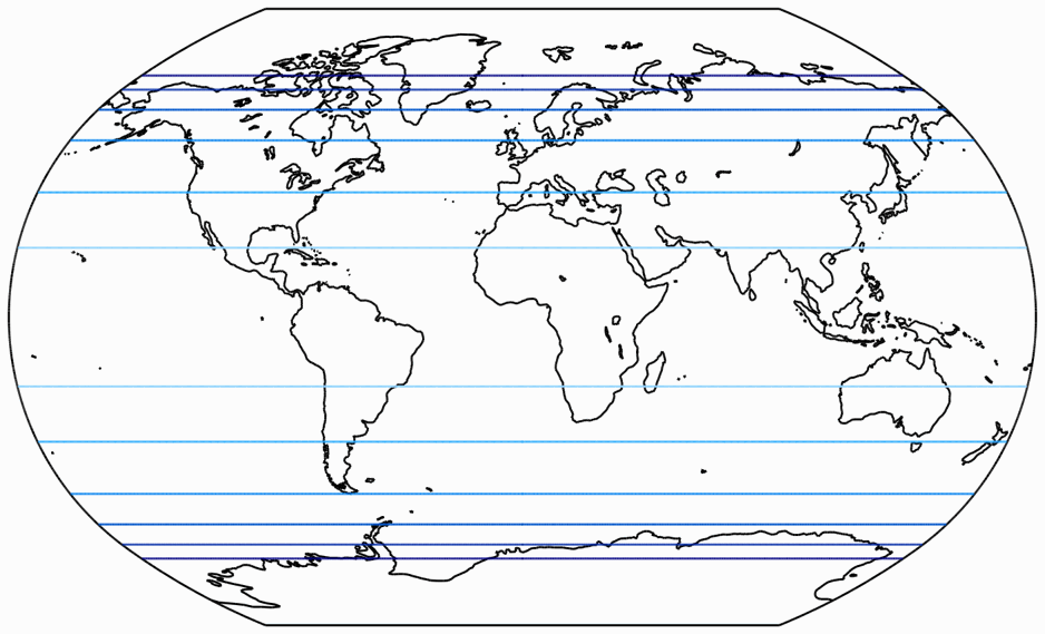
First the angular deformations,
the isolines are given for max. deformation of:
10°, 20°, 30°, 40°, 50°, and 60°.
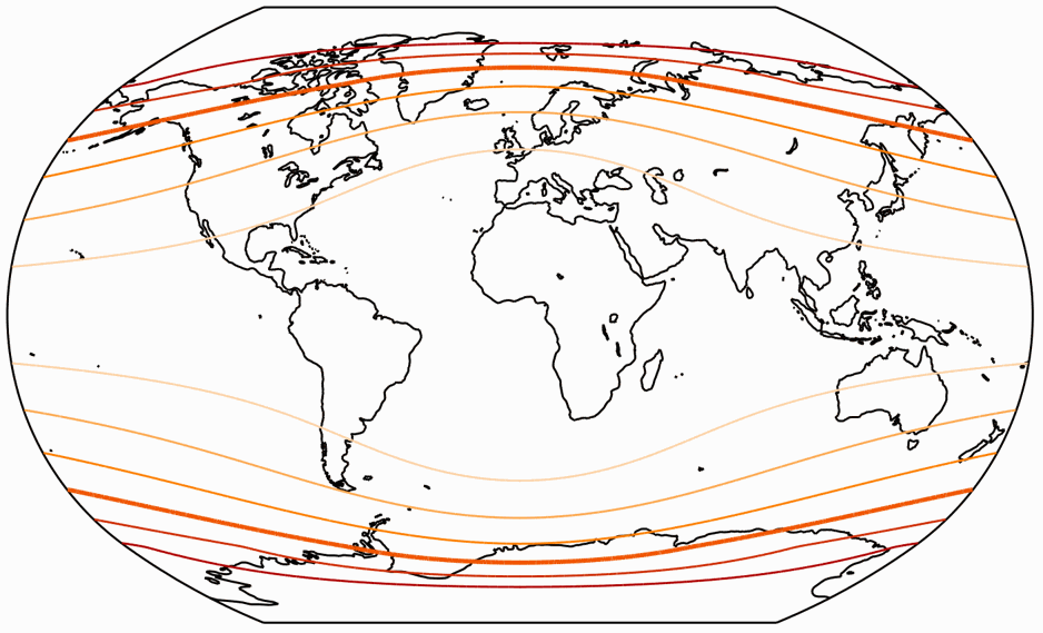
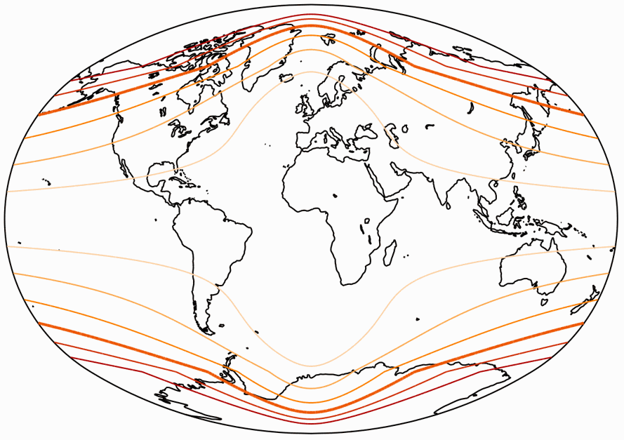
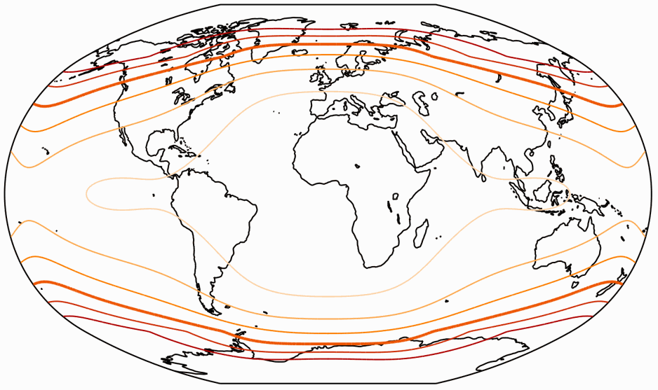

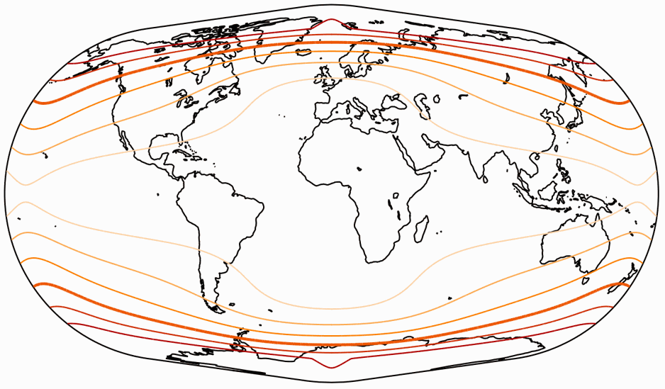

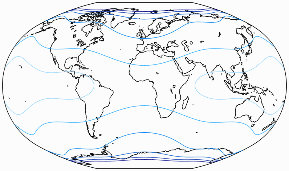
For the areal inflation, shown normalized to its minimum value,
the lines represent values of:
1.2; 1.5; 2.0; 2.5; 3.0; and 3.5.
The minimum value usually occurs at the central point, but for
Baranyi III to VII, it occurs where the equator meets the boundary.


A Very Convenient Mistake By Snyder
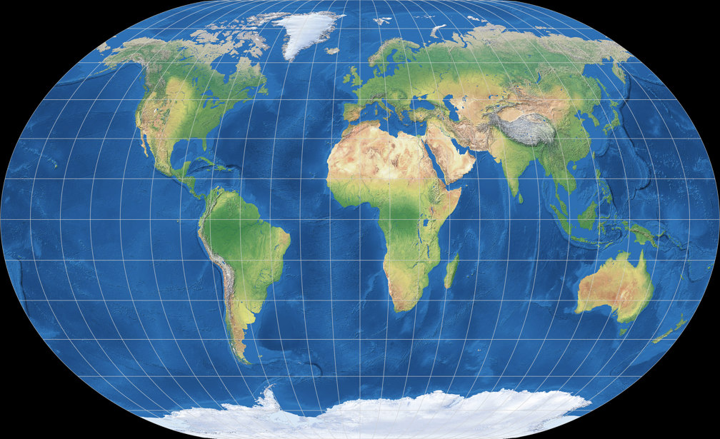
In 1977, John P. Snyder erroneously listed the Winkel II as the arithmetic mean of the Equirectangular and Mollweide projections (Apian II instead of Mollweide would be correct). He later rectified that mistake, and Evenden listed the Equirectangular/Mollweide version as Winkel-Snyder.[1][2]
So why is this a convenient mistake?
Because Winkel-Snyder is a very good pseudocylindric compromise projection!
I actually prefer it to Winkel II. But judge for yourself:
Winkel II vs. Winkel-Snyder.
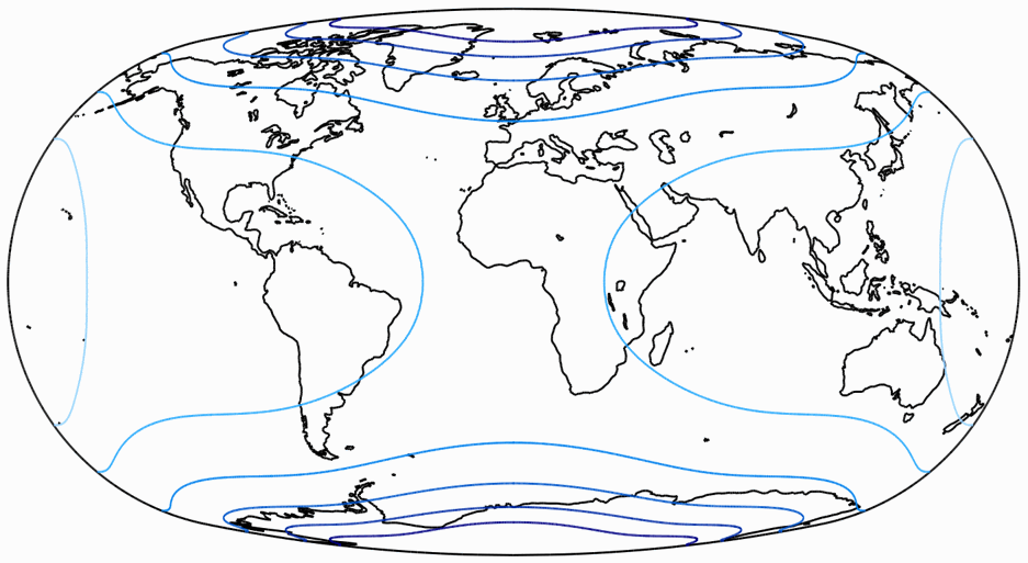
The distribution of the distortions is certainly not spectacular, but very decent:


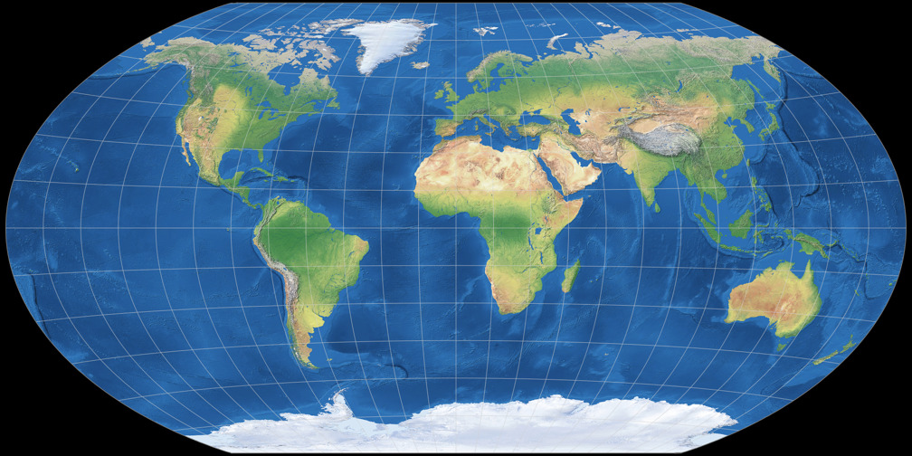
I talked about it before[3]: Oswald Winkel used a standard parallel of arccos(2/π) – or rounded 50°28´ – on the equirectangular projection before averaging. But of course you can set a different value here, as has been done on the Winkel Tripel, with 40° on the Winkel Tripel Bartholomew and 0°, i.e. the equator, on the Winkel Tripel BOPC. Two examples – Bartholomew’s 40°, transferred to the Winkel-Snyder; and with 28° as shown in a figure by Evenden (at least, approximately):


I think I’ll add one of them, or maybe both, to my Projection Collection soon.
There is another good thing about the Winkel-Snyder:
Although I had known about the it for a while, it was brought
to my attention again by
a comment in February,
and then… ah, I’m going to talk about that soon. And maybe you already know about it anyway.
Bis die Tage!
References / Footnotes
-
↑
Snyder, John P.:
Flattening the Earth: Two Thousand Years of Map Projections.
Chicago 1993, page 307. -
↑
Evenden, Gerald I.:
libproj4 manual
Falmouth 2008, page 66. - ↑ See my blogpost Happy Birthday, Winkel Tripel! of May 2021.
 Except where otherwise noted, images on this site are licensed under
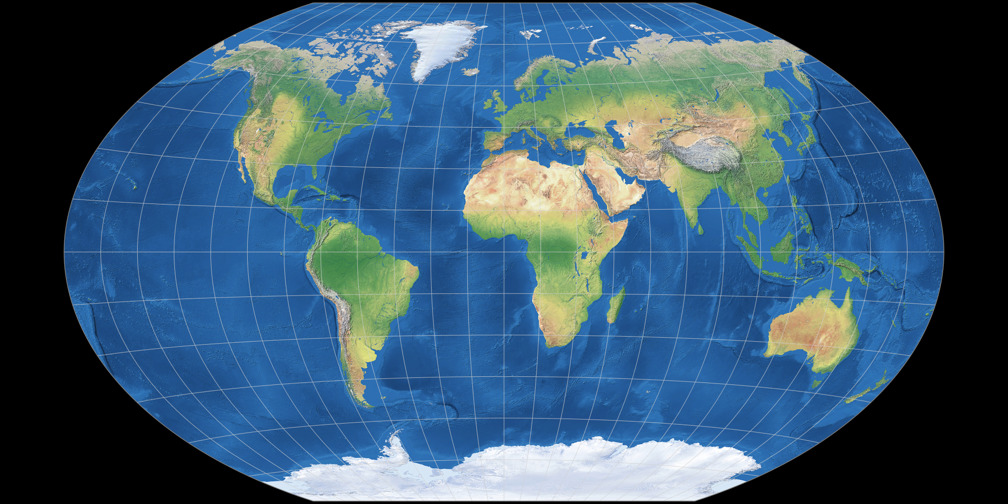
Comments
Due to spam posts, comments are now subject to moderation, which means they remain hidden until they are approved by a moderator.
More info
Be the first one to write a comment!